蚁群算法
蚁群算法(Ant Colony Optimization, ACO) 是一种基于群体智能的元启发式算法,灵感来源于蚂蚁觅食行为。蚂蚁在寻找食物时,会通过释放信息素(pheromone)来标记路径,其他蚂蚁会根据信息素的浓度选择路径。通过模拟这一行为,ACO 可以有效地解决组合优化问题,如旅行商问题(TSP)。
蚁群算法的基本思想
蚂蚁的路径选择:
- 每只蚂蚁根据信息素浓度和启发式信息(如距离)选择下一个要访问的城市。
- 信息素浓度越高,路径被选择的概率越大。
信息素更新:
- 蚂蚁完成一次遍历后,会根据路径的长度更新信息素。
- 路径越短,信息素增加得越多。
正反馈机制:
- 信息素的积累和挥发形成正反馈机制,使得较优路径的信息素浓度逐渐增加。
TSP问题描述
假设有n个城市,城市之间的距离用一个距离矩阵$D$表示, $D_{ij}$表示城市i,j之间的距离。目标是找到一个路径或排列$\pi=(\pi_1,\pi_2, …, \pi_n)$,使得以下总距离最小:
蚁群算法解决 TSP 的步骤
初始化:
- 初始化信息素矩阵$\tau$,通常设置为一个较小的常数。
- 初始化启发式信息矩阵 $ \eta $,通常为距离的倒数 $ \eta{ij} = \frac{1}{D{ij}} $。
蚂蚁的路径构建:
- 每只蚂蚁从起点出发,根据概率选择下一个城市,直到访问完所有城市。
- 单只蚂蚁选择概率公式:其中:
- $ \tau_{ij} $ 是信息素浓度。
- $ \eta_{ij} $ 是启发式信息。
- $ \alpha $ 和 $ \beta $ 是控制信息素和启发式信息权重的参数。
信息素更新:
- 所有蚂蚁(蚂蚁有m只)完成各自路径构建后,更新信息素:其中:
- $ \rho $ 是信息素挥发率。
- $ \Delta \tau_{ij}^k $ 是第 $ k $ 只蚂蚁在路径 $ (i, j) $ 上释放的信息素,通常与路径长度成反比:
- $ Q $ 是常数。
- $ L_k $ 是蚂蚁 $ k $ 的走过的路径长度。
迭代:
- 重复路径构建和信息素更新过程,直到达到最大迭代次数或找到满意解。
代码实现(Python)
以下是使用蚁群算法解决 TSP 的 Python 实现:
1
2
3
4
5
6
7
8
9
10
11
12
13
14
15
16
17
18
19
20
21
22
23
24
25
26
27
28
29
30
31
32
33
34
35
36
37
38
39
40
41
42
43
44
45
46
47
48
49
50
51
52
53
54
55
56
57
58
59
60
61
62
63
64
65
66
67
68
69
70
71
72
73
74
75
76
77
78
79
80
81
82
83
84
85
86
87
88
89
90
91
92
93
94
95
96
97
98
99
100
101
102
103
| import numpy as np
class AntColony:
def __init__(self, distances, n_ants, n_iterations, decay, alpha=1, beta=2):
"""
初始化参数:
- distances: 距离矩阵
- n_ants: 蚂蚁数量
- n_iterations: 迭代次数
- decay: 信息素挥发率
- alpha: 信息素权重
- beta: 启发式信息权重
"""
self.distances = distances
self.n_ants = n_ants
self.n_iterations = n_iterations
self.decay = decay
self.alpha = alpha
self.beta = beta
self.n_cities = len(distances)
self.pheromone = np.ones((self.n_cities, self.n_cities))
def run(self):
best_path = None
best_distance = float('inf')
for iteration in range(self.n_iterations):
all_paths = self._build_paths()
self._update_pheromone(all_paths)
shortest_path = min(all_paths, key=lambda x: x[1])
if shortest_path[1] < best_distance:
best_distance = shortest_path[1]
best_path = shortest_path[0]
print(f"Iteration {iteration + 1}: Best Distance = {best_distance}")
return best_path, best_distance
def _build_paths(self):
all_paths = []
for _ in range(self.n_ants):
path = self._build_single_path()
distance = self._calculate_distance(path)
all_paths.append((path, distance))
return all_paths
def _build_single_path(self):
path = []
visited = set()
start_city = np.random.randint(self.n_cities)
path.append(start_city)
visited.add(start_city)
while len(visited) < self.n_cities:
next_city = self._choose_next_city(path[-1], visited)
path.append(next_city)
visited.add(next_city)
return path
def _choose_next_city(self, current_city, visited):
probabilities = []
for city in range(self.n_cities):
if city not in visited:
pheromone = self.pheromone[current_city][city]
distance = self.distances[current_city][city]
probabilities.append((pheromone ** self.alpha) * ((1 / distance) ** self.beta))
else:
probabilities.append(0)
probabilities = np.array(probabilities)
probabilities /= probabilities.sum()
next_city = np.random.choice(range(self.n_cities), p=probabilities)
return next_city
def _calculate_distance(self, path):
distance = 0
for i in range(len(path) - 1):
distance += self.distances[path[i]][path[i + 1]]
distance += self.distances[path[-1]][path[0]]
return distance
def _update_pheromone(self, all_paths):
self.pheromone *= (1 - self.decay)
for path, distance in all_paths:
for i in range(len(path) - 1):
self.pheromone[path[i]][path[i + 1]] += 1 / distance
self.pheromone[path[-1]][path[0]] += 1 / distance
distances = np.array([
[0, 10, 15, 20],
[10, 0, 35, 25],
[15, 35, 0, 30],
[20, 25, 30, 0]
])
ant_colony = AntColony(distances, n_ants=10, n_iterations=100, decay=0.1, alpha=1, beta=2)
best_path, best_distance = ant_colony.run()
print("Best Path:", best_path)
print("Best Distance:", best_distance)
|
参数说明
- 蚂蚁数量(n_ants):蚂蚁数量越多,搜索能力越强,但计算成本也越高。
- 迭代次数(n_iterations):迭代次数越多,算法越有可能找到更优解。
- 信息素挥发率(decay):控制信息素的挥发速度,通常取值在 0.1 到 0.5 之间。
- 信息素权重(alpha):控制信息素对路径选择的影响。
- 启发式信息权重(beta):控制启发式信息(如距离)对路径选择的影响。
总结
- 蚁群算法是一种基于群体智能的优化算法,适合解决 TSP 等组合优化问题。
- 通过模拟蚂蚁觅食行为,算法能够逐步找到较优解。
- 算法的性能受参数设置影响较大,需要根据具体问题进行调整。
- 蚁群算法的优势在于其并行性和鲁棒性,适合解决大规模复杂问题。
退火算法
模拟退火算法(Simulated Annealing, SA) 是一种基于概率的全局优化算法,灵感来源于固体退火过程。它通过引入“温度”参数和概率接受机制,能够在搜索过程中跳出局部最优解,逐步逼近全局最优解。模拟退火算法非常适合解决组合优化问题,如旅行商问题(TSP)。
模拟退火算法的基本思想
- 初始解:从一个初始解(例如随机路径)开始。
- 邻域搜索:在当前解的邻域中生成一个新解。
- 接受准则:
- 如果新解比当前解更优,则接受新解。
- 如果新解比当前解差,则以一定概率接受新解。概率由以下公式决定:其中:
- $\Delta E$ 是新解与当前解的目标函数值差。
- $T$ 是当前温度。
- 降温:随着迭代次数增加,逐步降低温度 $T$。
- 终止条件:当温度降到某个阈值或达到最大迭代次数时,算法结束。
模拟退火算法解决 TSP 的步骤
以下是使用模拟退火算法解决 TSP 的具体步骤:
1. 初始化
- 生成一个初始路径(例如随机排列)。
- 设置初始温度 $T_0$ 和降温速率 $\alpha$。
- 设置终止温度 $T_{\text{min}}$ 和最大迭代次数。
2. 邻域搜索
在当前路径的邻域中生成一个新路径。常用的邻域操作包括:
- 交换:随机选择两个城市并交换它们的位置。
- 逆序:随机选择一段路径并逆序排列。
- 插入:随机选择一个城市并插入到另一个位置。
3. 接受准则
计算新路径的总距离 $E{\text{new}}$ 和当前路径的总距离 $E{\text{current}}$:
- 如果 $E{\text{new}} < E{\text{current}}$,接受新路径。
- 如果 $E{\text{new}} \geq E{\text{current}}$,以概率 $P = \exp\left(-\frac{E{\text{new}} - E{\text{current}}}{T}\right)$ 接受新路径。
4. 降温
更新温度:
其中 $\alpha$ 是降温速率(通常取 $0.8 \leq \alpha \leq 0.99$)。
5. 终止条件
当温度降到 $T_{\text{min}}$ 或达到最大迭代次数时,算法结束。
代码实现(Python)
以下是使用模拟退火算法解决 TSP 的 Python 实现:
1
2
3
4
5
6
7
8
9
10
11
12
13
14
15
16
17
18
19
20
21
22
23
24
25
26
27
28
29
30
31
32
33
34
35
36
37
38
39
40
41
42
43
44
45
46
47
48
49
50
51
52
53
54
55
56
57
58
59
60
61
62
63
64
65
66
67
68
69
70
71
72
73
74
| import math
import random
def calculate_distance(path, distances):
distance = 0
for i in range(len(path) - 1):
distance += distances[path[i]][path[i + 1]]
distance += distances[path[-1]][path[0]]
return distance
def generate_initial_path(n_cities):
path = list(range(n_cities))
random.shuffle(path)
return path
def swap_cities(path):
new_path = path.copy()
i, j = random.sample(range(len(path)), 2)
new_path[i], new_path[j] = new_path[j], new_path[i]
return new_path
def simulated_annealing(distances, T0=1000, alpha=0.99, T_min=1e-3, max_iter=1000):
n_cities = len(distances)
current_path = generate_initial_path(n_cities)
current_distance = calculate_distance(current_path, distances)
best_path = current_path.copy()
best_distance = current_distance
T = T0
for iteration in range(max_iter):
if T < T_min:
break
new_path = swap_cities(current_path)
new_distance = calculate_distance(new_path, distances)
delta_E = new_distance - current_distance
if delta_E < 0 or random.random() < math.exp(-delta_E / T):
current_path = new_path
current_distance = new_distance
if current_distance < best_distance:
best_path = current_path.copy()
best_distance = current_distance
T *= alpha
if iteration % 100 == 0:
print(f"Iteration {iteration}: Best Distance = {best_distance}, Temperature = {T}")
return best_path, best_distance
distances = [
[0, 10, 15, 20],
[10, 0, 35, 25],
[15, 35, 0, 30],
[20, 25, 30, 0]
]
best_path, best_distance = simulated_annealing(distances)
print("Best Path:", best_path)
print("Best Distance:", best_distance)
|
参数说明
- 初始温度 $T_0$:控制初始接受劣解的概率,通常设置为一个较大的值(如 1000)。
- 降温速率 $\alpha$:控制温度的下降速度,通常取 $0.8 \leq \alpha \leq 0.99$。
- 终止温度 $T_{\text{min}}$:当温度降到该值时,算法停止。
- 最大迭代次数:算法的最大运行次数。
总结
- 模拟退火算法是一种全局优化算法,适合解决 TSP 等组合优化问题。
- 通过引入温度和概率接受机制,算法能够跳出局部最优解,逐步逼近全局最优解。
- 算法的性能受参数设置影响较大,需要根据具体问题进行调整。
- 模拟退火算法的优势在于其简单性和鲁棒性,适合解决中小规模问题。
订单拣选问题
问题概述:
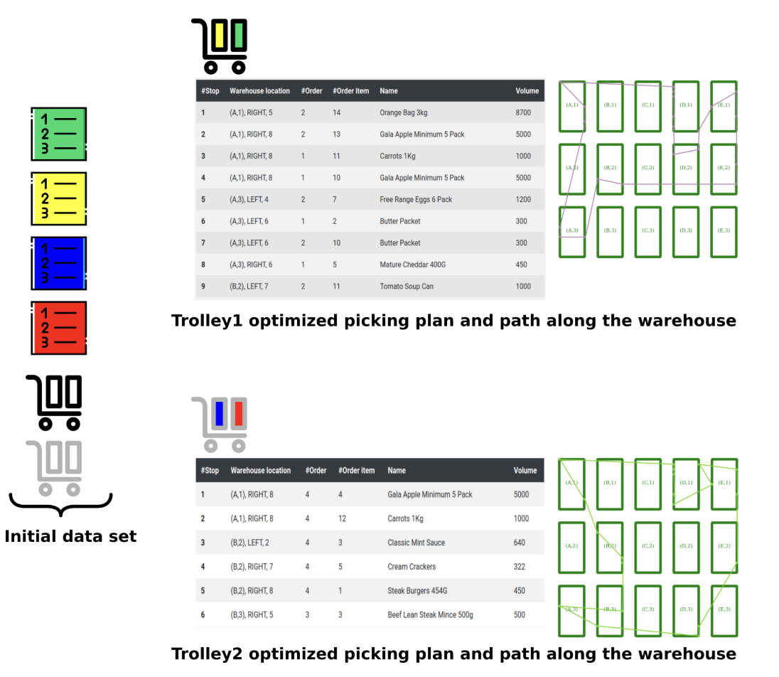
订单拣选问题由一组需要准备交付给不同客户的订单组成。每个订单都由一组订单项目(请求的产品)组成。这些产品位于仓库或超市的货架上,并占用特定体积的空间。为了完成订单,超市中有一组可用的手推车,它们遵循计算的路径并拣选订单项目。在此路径的每个步骤中选取一个订单项。产品在仓库中的位置决定了手推车的路径,每个手推车中的空间被划分为多个具有指定容量的桶。订单拣选问题的目标是计算一个拣选计划,该计划为每个手推车提供路径并考虑以下约束:
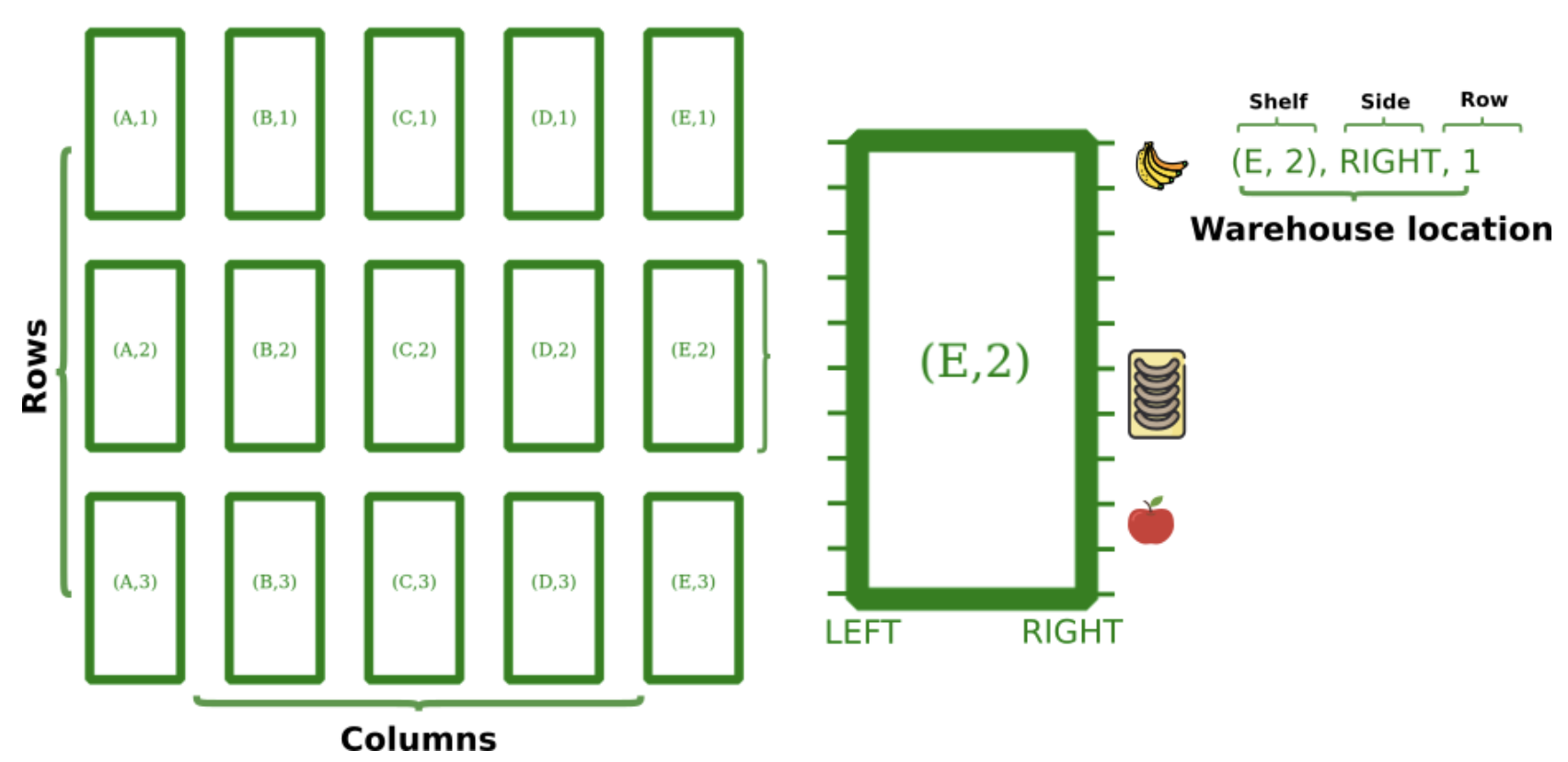
为了表述问题,仓库被定义为一组组织成列和行的货架。商品位于特定货架的左侧或右侧的特定行上。货架、侧边和行决定了产品位置。
博客https://www.optaplanner.org/blog/2021/10/14/OrderPickingQuickstart.html
类比到智能巡检排程项目:
- 订单:检修任务
- 订单项:检修部件,检修的部件占用一定的发电损失,检修部件位于风场的风机上。
- 手推车:检修人员。
- 手推车行驶距离最小:发电量损失最小。
- 不同部件不得同一时间让同一个检修员检修。
- 同一风机的所有部件检修完前不得检修另一个风机的部件。